Point Morphology
Seminar Project
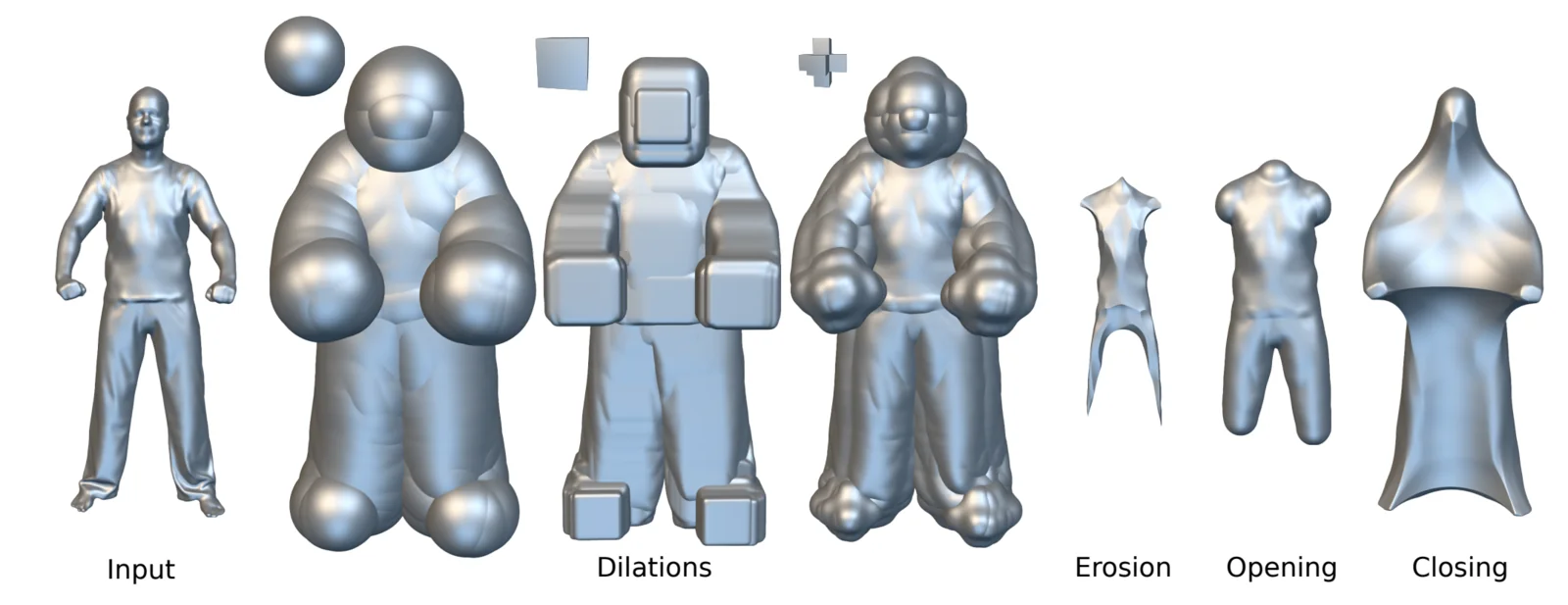
Morphology as a shape transformation method typically is defined in terms of supersets of input point sets. If repeated applications of morphological operations are required, approaches relying on supersets become impractical due to a failue to capture sharp features and their computational complexity. The proposed method which relies on projection and sampling sampling strategies aims to address these challenges.
Mathematical Morphology
Mathematical Morphology is a framework for shape transformation based on operations between sets. Given a shape and a Structuring Element (SE), operations such as dilation and erosion are defined by dragging the SE along the boundary of the input shape, either extruding or eroding it accordingly. This process is visualized below. The classical formulation relies on the Minkowski addition, which operates directly on sets and is computationally expensive by nature. The method presented in the following sections aims to improve performance by restricting computation to a point sampling of the surface, avoiding the overhead of full set-based representations.
2D Morphology


Images via Wikipedia – Mathematical Morphology (CC BY-SA)
Morphological Projection
The core contribution of the paper is a reformulation of morphological operations as a projection onto a Point Structuring Element (PSE). Rather than computing Minkowski sums, the method projects surface points onto a PSE that is fitted to the original surface, approximating dilation and erosion in a purely point-based setting.
Point Structuring Element
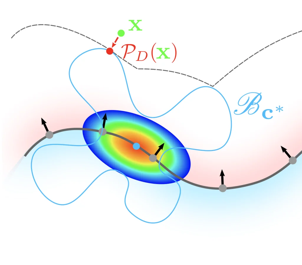
PSE centered at \(\mathbf{c^*}\) on the surface and the desired (dilated) projection onto the boundary \(\mathcal{P}_D\)
The PSE is the primtive or brush which defines the local shape used in morphological operations. It is the analogue of the classical SE but defined in an implicit form. A scaled and translated PSE is defined as:
$$\mathscr{B}_\mathbf{c}(\mathbf{x}) = s \, \mathscr{B}\left(\frac{\mathbf{x} - \mathbf{c}}{s}\right)$$
where \(s\) controls the scale of the structuring element, \(\mathbf c\) denotes its center and \(\mathscr{B}\) is the variational representation of the centered and normalized PSE shape (e.g. for a sphere \(\mathscr B(\mathbf x) = \|\mathbf x\|_2 - 1\)). This formulation measures the signed distance from any point \(\mathbf x\) to the boundary of the PSE. A formulation like this will become important since it allows us to define a projection operator \(\mathcal P\) that can take a point in space and project it right onto the boundary given that we can evaluate the gradient of our PSE:
$$\mathcal P(\mathbf x) = \mathbf x - \mathscr B_{\mathbf c} (\mathbf x) \frac{\nabla \mathscr B_{\mathbf c}(\mathbf x)}{\|\nabla \mathscr B_{\mathbf c}(\mathbf x)\|}$$
Fitting
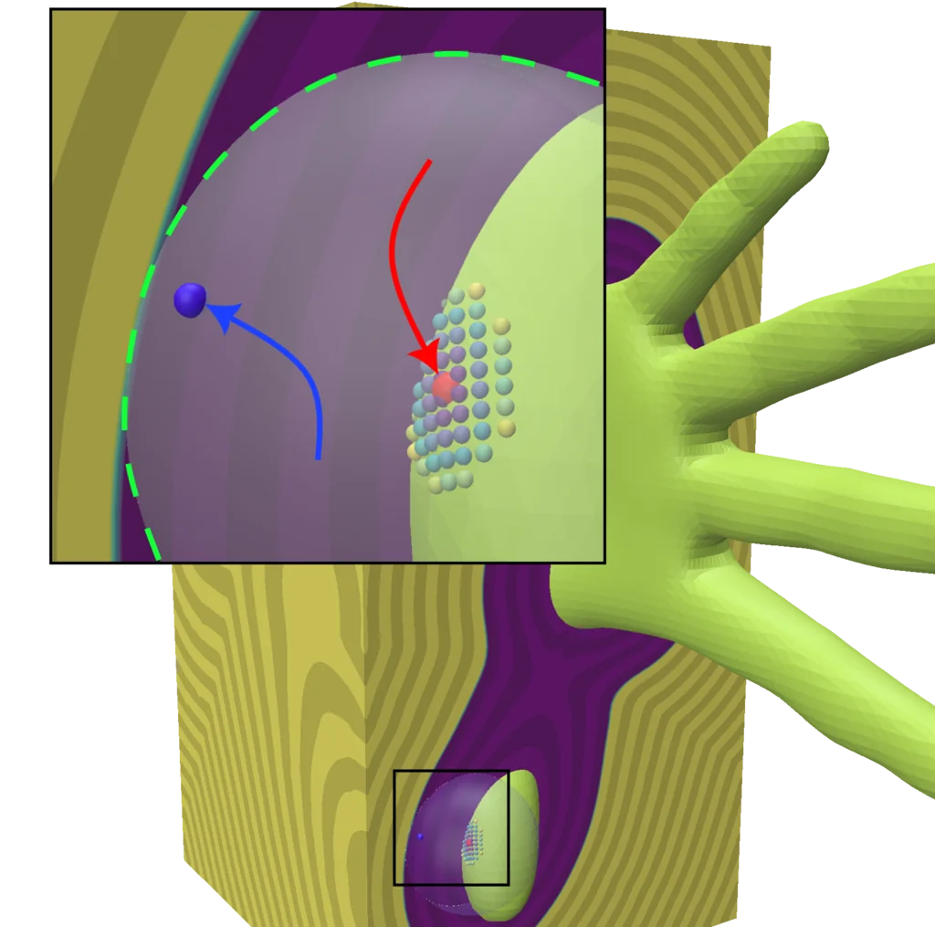
Find optimal center \(\color{red}{\mathbf{c^*}(\mathbf x)}\) as weigthed mean of surface samples in neighbourhood of \(\color{blue}{\mathbf{x}}\) defining the PSE boundary \(\color{limegreen}{\mathscr{B}}\)
To actually perform a projection onto a PSE which conforms to our notion of Morphology we need to ensure that the PSE is centered at the correct postion on the original surface. For this purpose we introduce the notion of a fitted PSE centered at optimal location \(\mathbf{c^*}\). We say that for a point of interest \(\mathbf x\), a PSE is fitted if:
$$\DeclareMathOperator*{\argmin}{argmin} \mathbf{c^*}(\mathbf x) = \argmin_{\mathscr{I}(\mathbf c) = 0} \mathscr{B}_{\mathbf c}(\mathbf x)$$
With \(\mathscr I\) the implicit function defining our original input surface. Essentially, we slide the PSE along our surface until the distance from our point to its boundary is minimized. As it stands this is a global optimization problem with a nonlinear constraint. To solve this problem we can reformulate it as a maximization of a weighted kernel-density estimation (KDE)
$$ \DeclareMathOperator*{\argmax}{argmax} \mathbf{c^*}(\mathbf x) = \argmax_{\mathbf c \in \mathbb{R}^3 \, \mathscr{I}(\mathbf p_i) = 0} \sum_i \underbrace{ \omega_\sigma(\mathscr{B}_{\mathbf p_i}(\mathbf x)) }_{\text{weighting}} \underbrace{ \omega_\sigma(\|\mathbf c - \mathbf p_i \|_2) }_{\text{kernel (standard KDE)}} $$
where \(\mathscr B\) functions as our weighting wrapped by a gaussian which turns our problem into a maximization problem. Written in this form we can use the mean-shift procedure to obtain a candiate that maximizes our new objective.
Iterative Projection
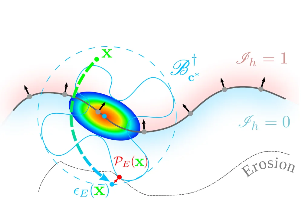
PSE projection of point \(\mathbf x\) outside the surface is prepended by the Erosion shift \(\epsilon_E\) in order to reach the erosion boundary
Actually the projection operator so far does not tell the whole story, since the projection result is dependent on the original point \(\mathbf x\) we start with, to which the optimal center \(\mathbf{c^*}\) is fitted. Further, given that we want to perform either a Dilation or an Erosion we want the make sure that we always project outwards/inwards.
To tackle this, a shift operation \(\epsilon\) is prepended, making sure that the point of interested is first moved close to the desired Morphological boundary, before being projected \[ \mathcal P_D = \mathcal P \circ \epsilon_D \\ \mathcal P_E = \mathcal P \circ \epsilon_E \] where \(\epsilon_D(\mathbf x) = \mathbf x + (1 - \mathscr I_h) \delta (\mathbf x)\) being the dilation shift operator, \(\mathscr I_h: \mathbb{R}^3 \rightarrow \{0, 1\}\) a indicator function giving \(\mathscr I_h(\mathbf x)= 1\) when \(\mathbf x\) is inside the surface.
To ensure a robust projection the final step is to repeat the projection until convergence: $$ \mathcal P_D^\infty = (\mathbf x) = \mathcal P_D \circ \dots \circ \mathcal P_D$$
Sampling
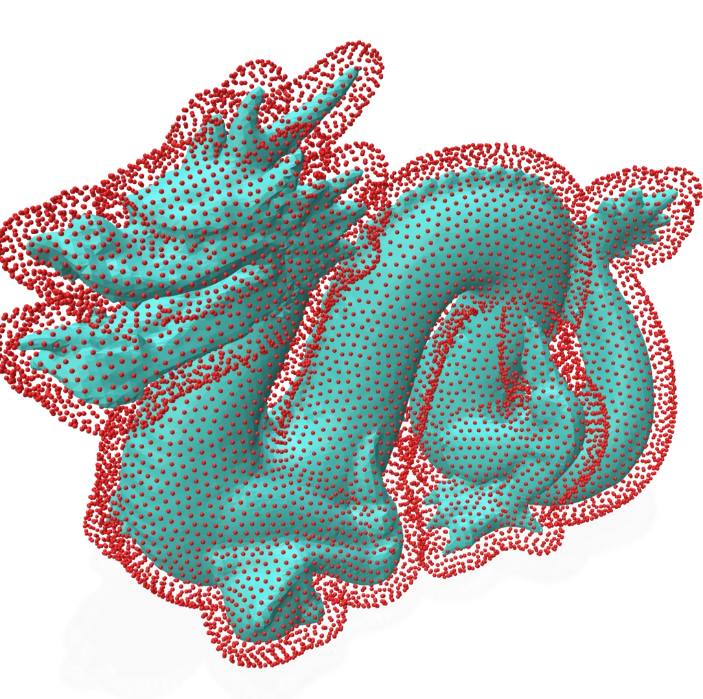
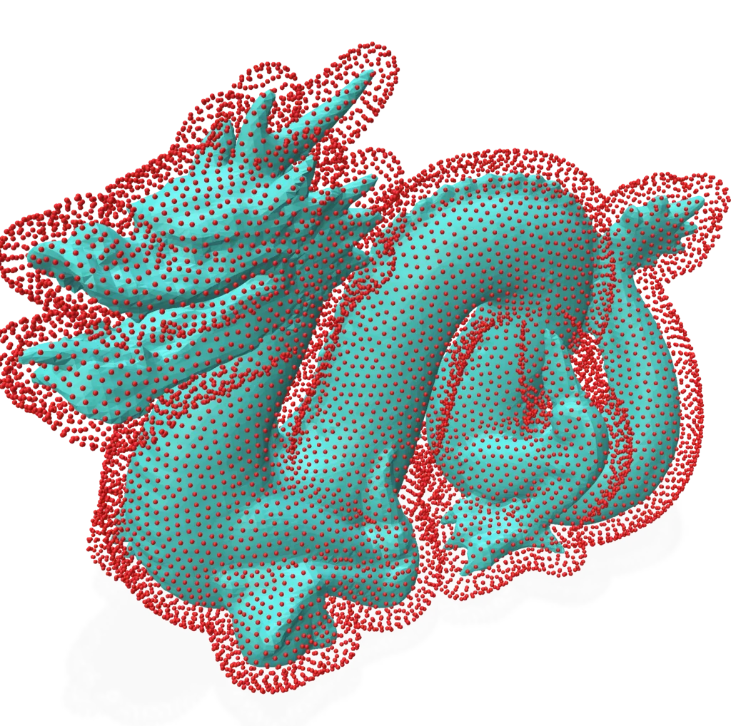
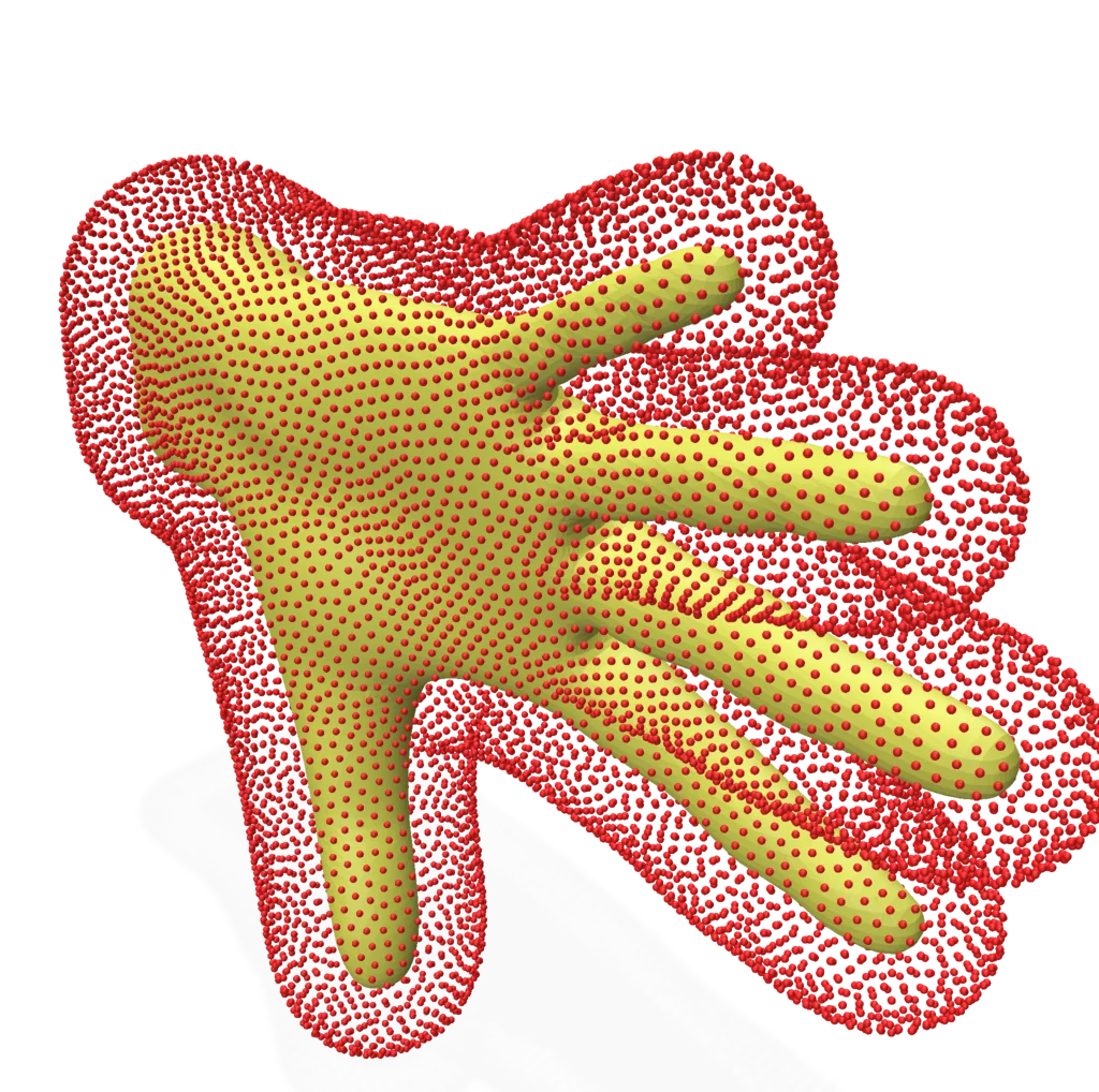
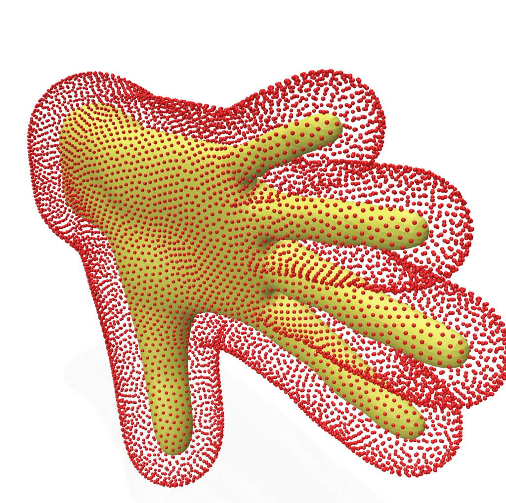
Naive sampling of the Morphological surface by starting with a dense set of points and performing the projection \(\mathcal P_D^\infty\) will leave us with point clusters and gaps on the surface (see Figure 1). To accurately represent the surface by some implicit surface model we aim to have points equally distributed across the surface while having more samples in regions with higher curvature. Taking results from [2] we can achieve this by filtering out duplicates thrugh subsampling (Figure 2) and finally moving the remaining points to undersampled regions thrugh resampling (Figure 3)
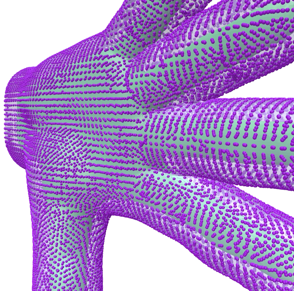
Initial dense sampling \(\Pi_{2D}\)
Figure 1
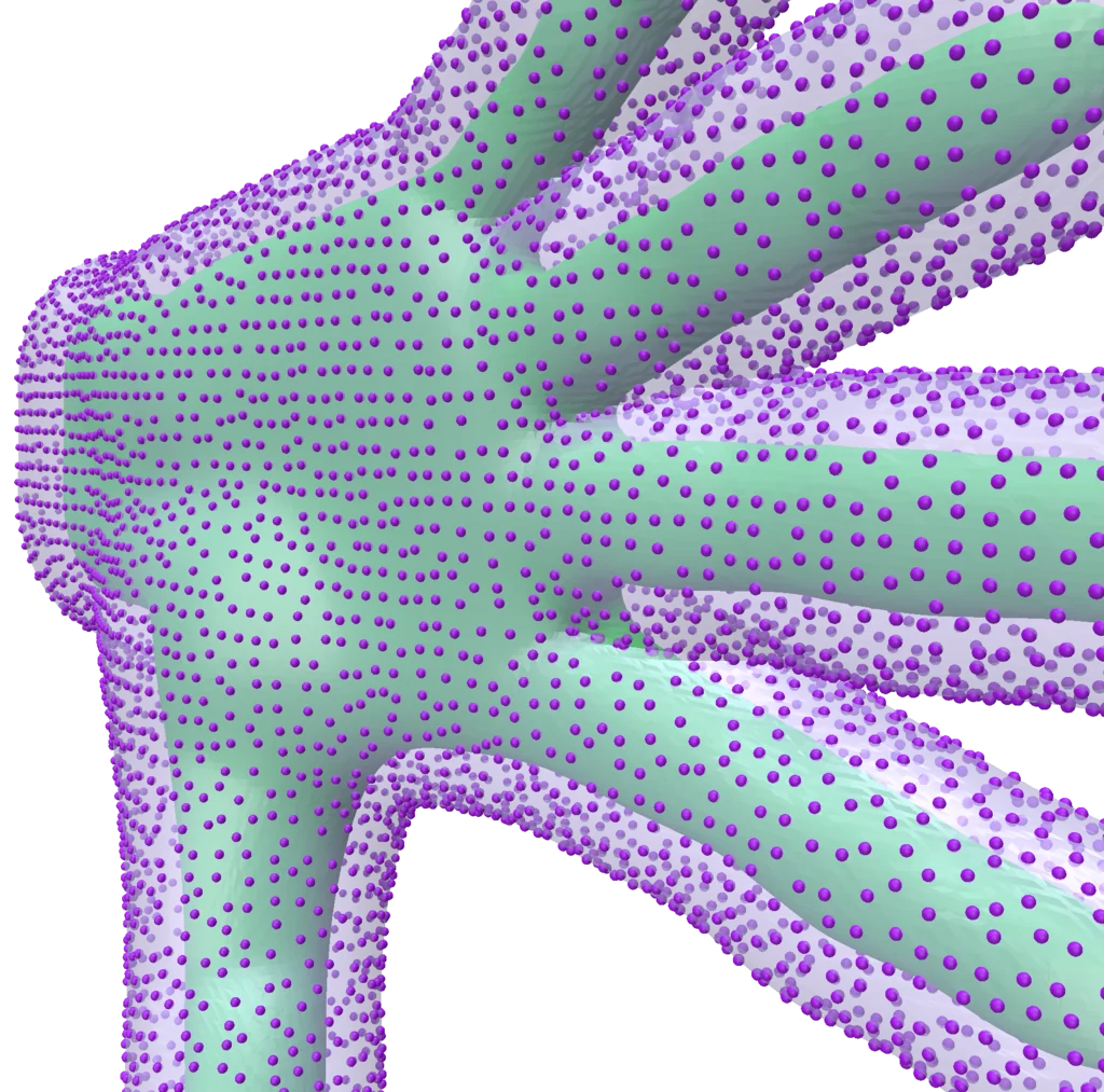
Subsampling
Figure 2
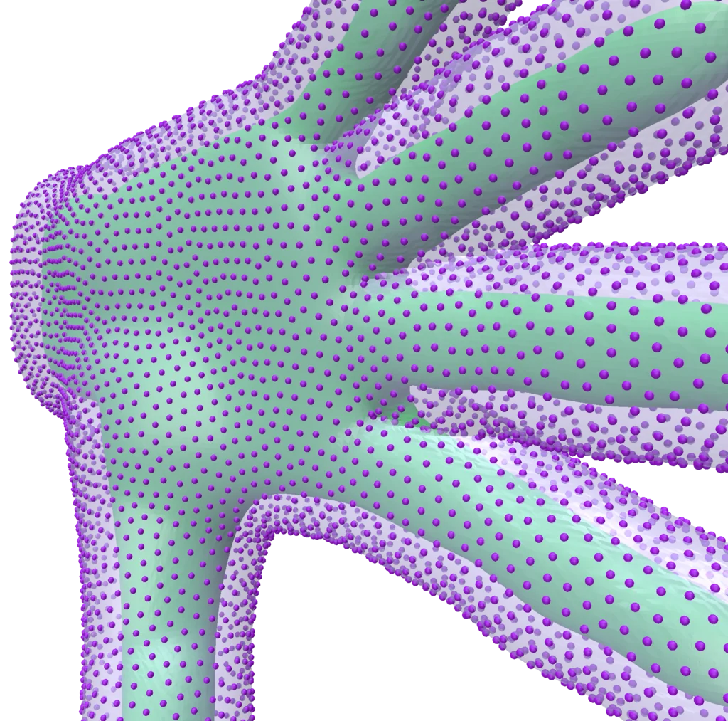
Morpho-adaptive sampling \( \Pi_{2D}^* \)
Figure 3
Point Importance Metric
Both subsampling and resampling as defined in [2] rely on evaluating an importance metric \(s(\mathbf{\hat x})\) for a point of interest on the surface. In the original paper this is defined as $$ s (\mathbf {\hat x}) = 1 - \mathbf k^T \mathbf K^{-1} \mathbf k $$ Where \(K_{ij} = k(\mathbf{\hat x}_i, \mathbf{\hat x}_j)\). and \(\mathbf{k}_i = k(\mathbf{\hat x}, \mathbf{\hat x}_i)\) and \(k\) a gaussian kernel. And we embed our position and fitted center in a feature space: $$\mathbf{\hat x} = \left[\frac{\mathbf x}{\sigma_p} \,\frac{\mathbf{c^*}(\mathbf x)}{\sigma_c}\right] \in \mathbb R^6$$ where \(\sigma_p, \sigma_c\) can be seen as controlling the width of a positional and centroid gaussian kernel respectively. E.g a larger value for \(\sigma_p\) leading to an enlarged region in which neighbours are considered simmilar, thus a sparser subsampling and therefore \(\sigma_p \propto\) the resulting point spacing of the output pointcloud.
Results
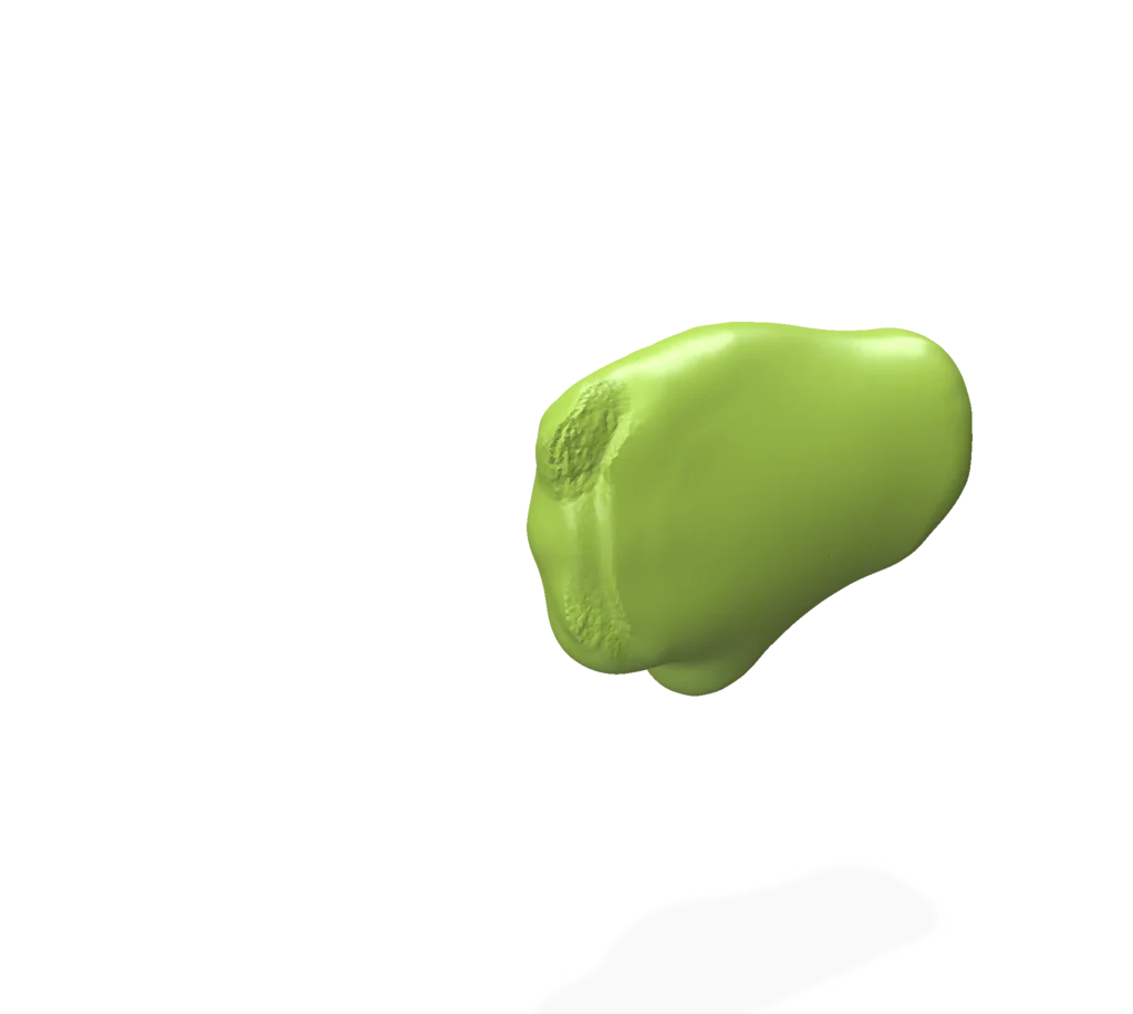
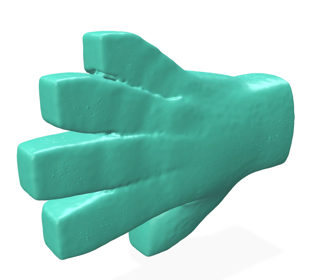
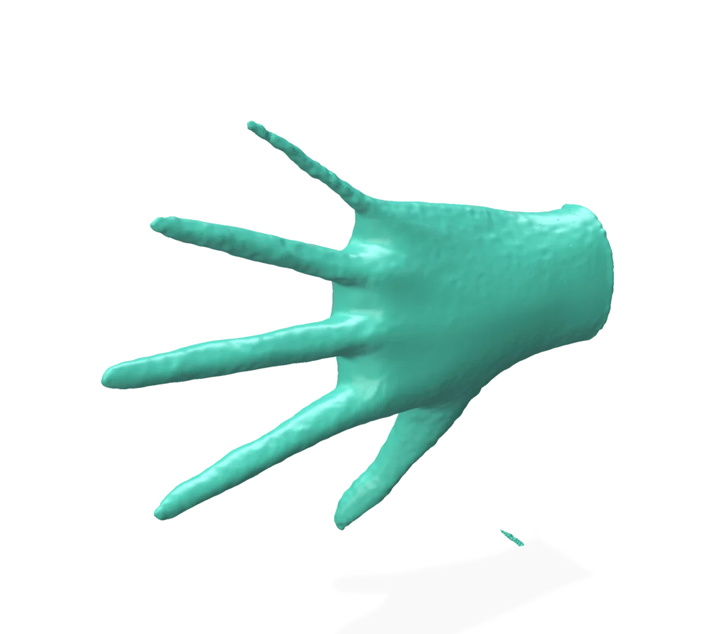
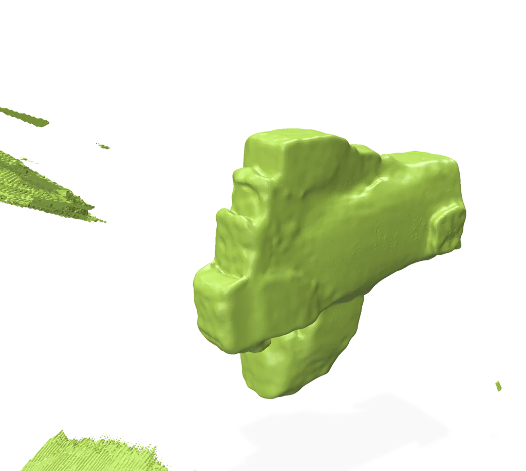
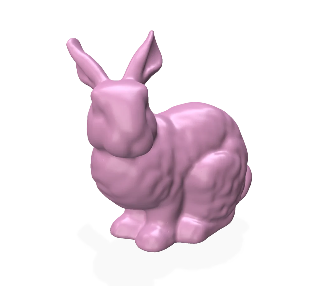
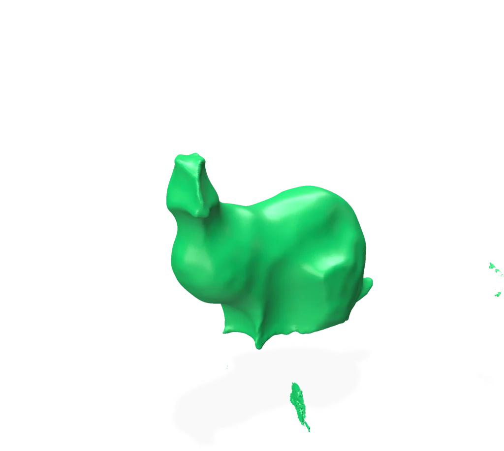
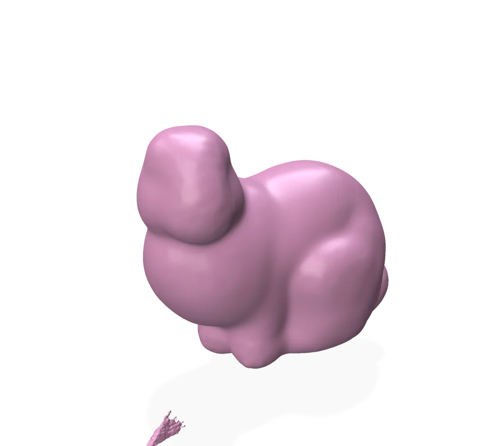
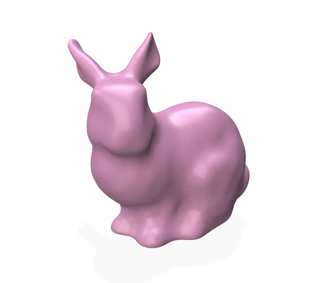
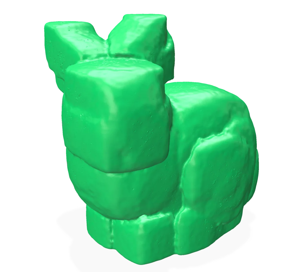
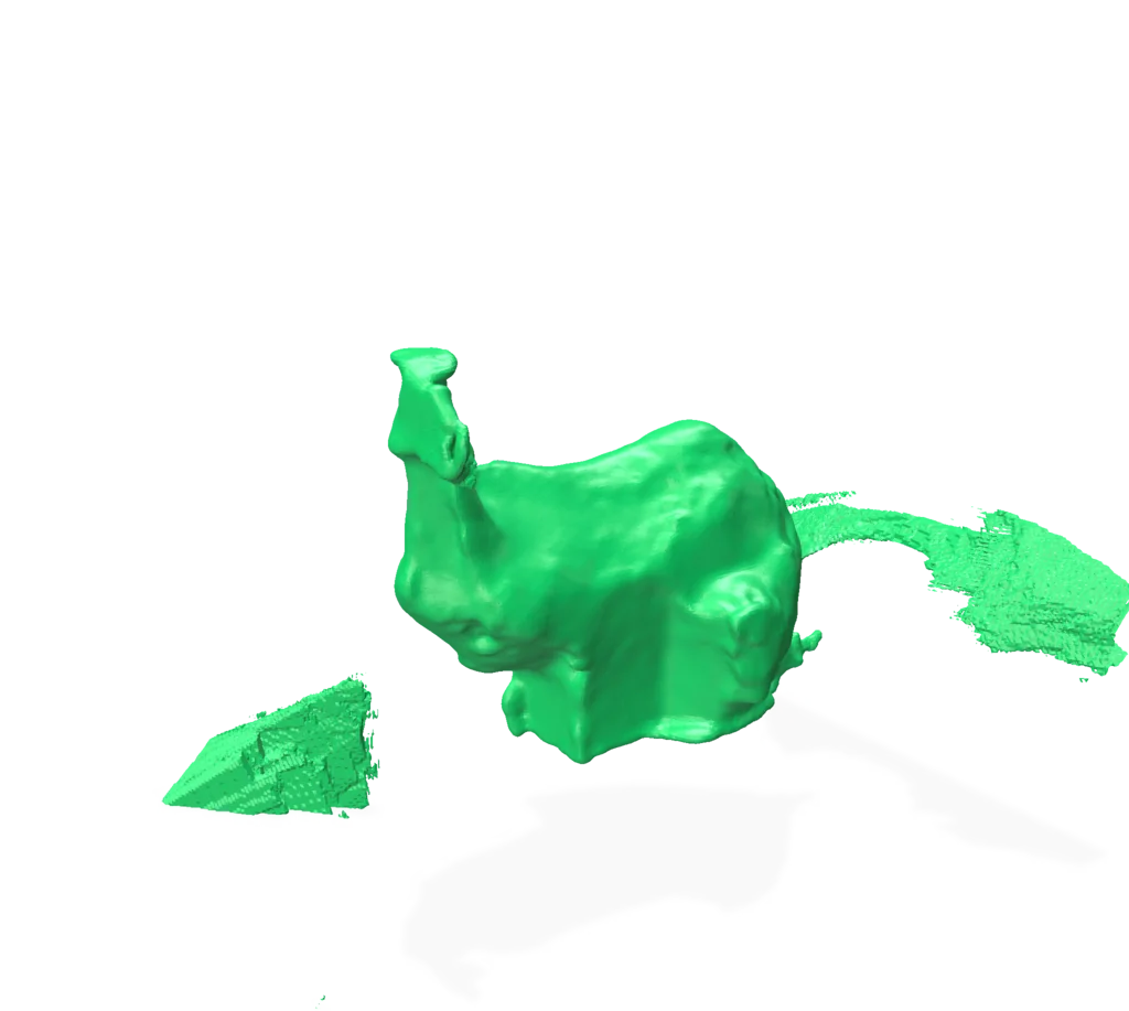
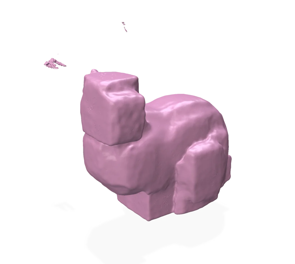
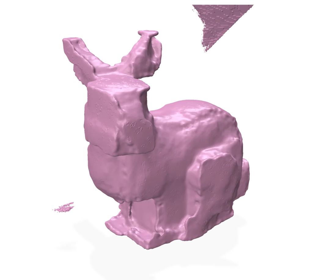
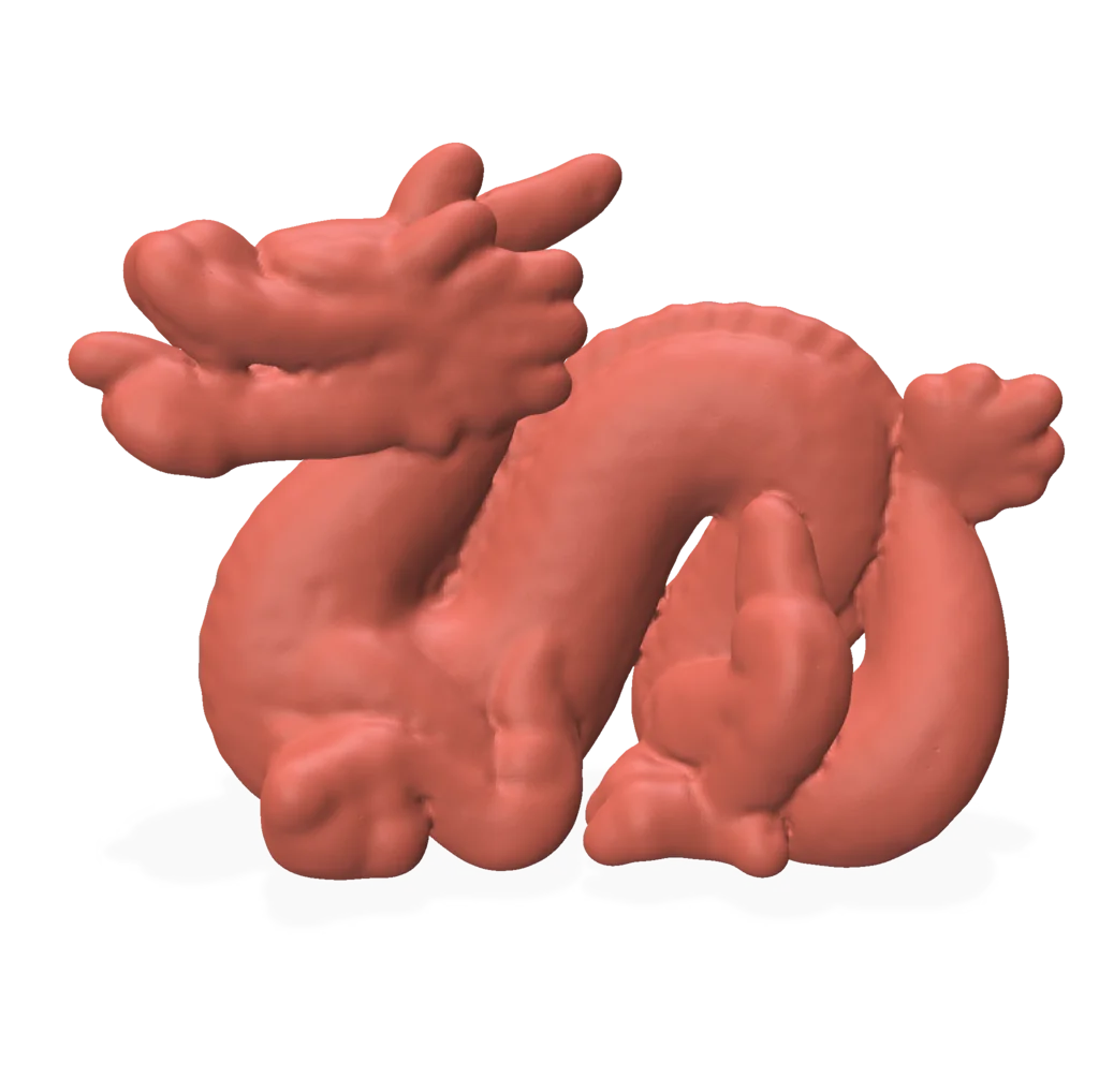
Results on three base models: Hand, Bunny, and Dragon for all morphological operations and two PSE shapes. The bounding box is scaled to have a diagonal length of 100. Feature-aware sampling was not used only morpho-adaptive resampling.
Select an operation and structuring element below. Hover any result card to compare against the input. Input
Input




 Input
Input

 Input
Input


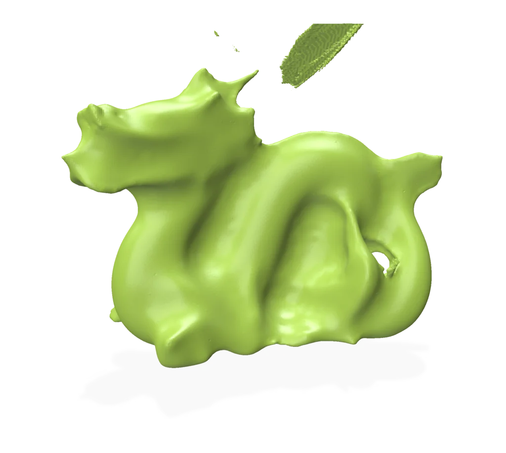
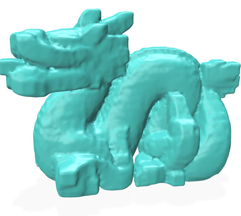

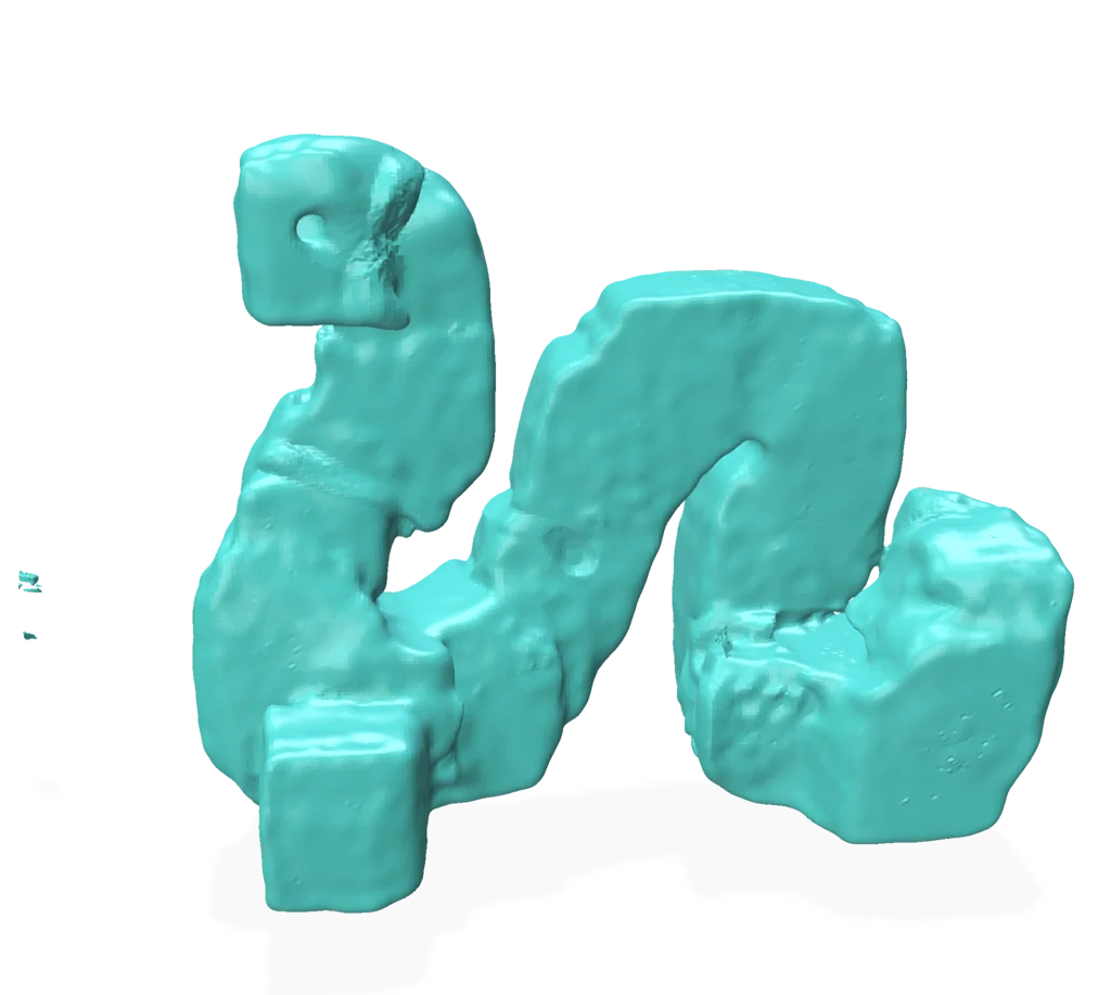
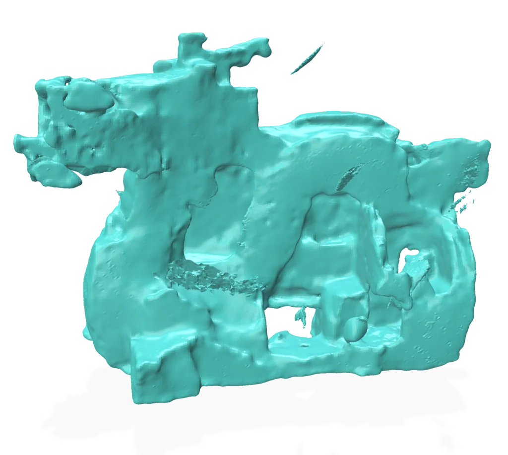
Discussion
The projection operator was straightforward to implement given its analytical form. The most significant implementation effort went into the importance metric used for subsampling and resampling, which was guided by the reference implementation of [2]. To serve as a readable learning resource, the source code is written to mirror the theory as closely as possible, with only limited performance optimization. This is clearly reflected in runtime when running morphology on dense point clouds. Most time is spent in the subsampling and resampling stage. The variational forms of the dilation and erosion operators: $$ D_{\mathscr{I},\mathscr{B}} = \min(\mathscr{B}_{\mathbf{c}^*}(\mathbf x), \mathscr{I}(\mathbf x)) \qquad E_{\mathscr{I},\mathscr{B}} = \max(-\mathscr{B}_{\mathbf{c}^*}(\mathbf x), \mathscr{I}(\mathbf x)) $$ was particularly efficient to implement, as it reduces to evaluating the iterative projection for any point on a grid followed by a min/max query. This representation provides a useful preview rendering of the target erosion or dilation, and in practice served as a guide for choosing parameters before running the full pipeline. Parameters such as the initial point spacing \(\sigma_p\) and the PSS support radius have a considerable impact on both performance and output quality.
Parameter coice
The guidance provided in the original papers regarding the relationship between structuring element size, initial point spacing, and PSS support radius can in practice be insufficient to avoid artifacts. For openings and closings in particular, the quality of the intermediate result is critical, as any noise in the PSS fit is amplified during the subsequent PSE fitting stage. Obtaining visually clean results therefore requires careful tuning and inspection of intermediate results. For the results the following parameter relationsips where chosen initially and potentially fine-tuned for cleaner results.
| Parameter | Role | Suggested value |
|---|---|---|
| \(\sigma\) | Support size of the MLS weighting kernel \(\omega_\sigma\); scale at which the PSS primitive is fitted to \(\Pi\) | Set to the kernel support of the input surface PSS; acts as an upper bound in the point-spacing rule for \(\sigma_p\) |
| \(\sigma_p\) | Width of the gaussian kernel applied to the positional component of our embedding space. A larger value resulting in a larger point spacing | \(\sigma_p = \min(\sigma,\, s)\,/\,2\), where \(s\) is the PSE minimum local feature size (e.g. radius for a spherical PSE) |
| \(\sigma_c\) | The width of the gaussian kernel comparing centroid positions. The
"morphological" distance from |
\(\sigma_c = s\) |
Artifacts
During testing, the iterative projection operator occasionally converged to points far from the surface, manifesting as outliers in the output point cloud and in turn introducing noise in the PSS representation. In [3] the authors note that the spherical fit can produce unwanted stationary points near the boundary of the surface definition domain. I did not implement the suggested mitigation strategy.
Sharp features introduced by erosion or dilation can lead to a locally noisy PSS representation, which is then amplified in subsequent pipeline stages such as opening and closing. Whether this reflects a fundamental limitation of the APSS implementation in capturing rapidly varying normals, or a wrong choice in parameters was often times hard to determine. One possibility for could be to incorporate dedicated sharp-edge handling as outlined in [3].
Morpho-adaptivity
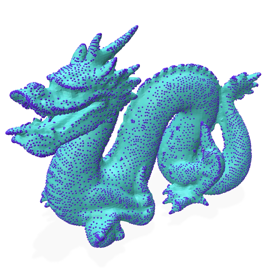
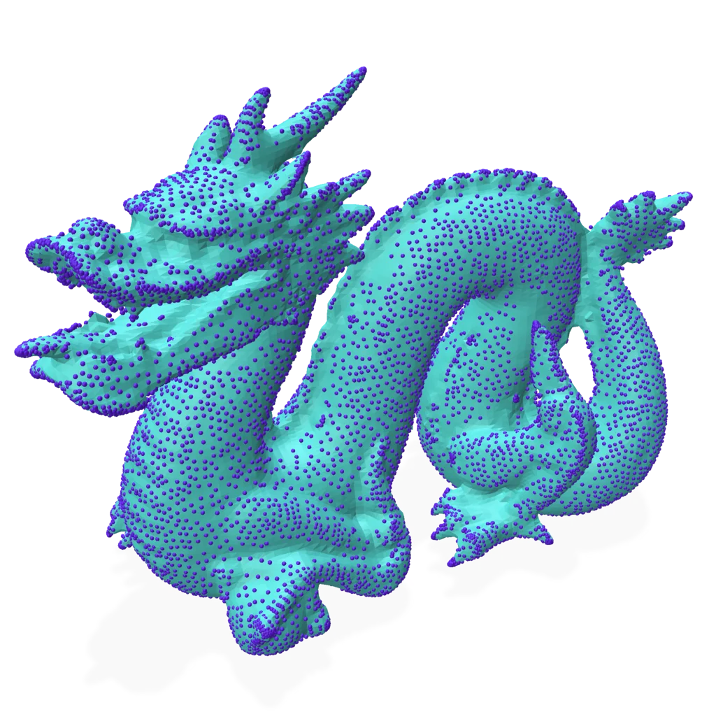
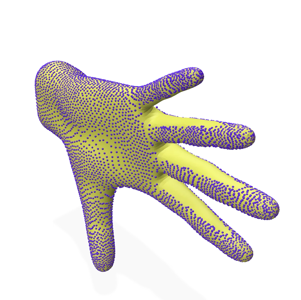
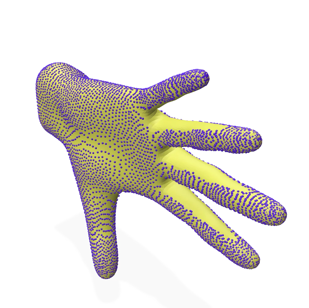
For computing the importance metric, the authors replaced the distance between normals with a distance between optimized centroids, with the goal of distributing samples more evenly across the original surface. In practice, this reformulation did not produce a noticeable difference. The stated motivation is “to distinguish samples that may be close in \(\mathbb{R}^3\) but belong to different surface regions (e.g., two sides of a thin sheet)”, but it is unclear why a normal-based distance would be insufficient for this purpose: on a thin sheet, normals on opposite sides differ substantially even when positions are close. The effect of the distance metric choice is visualized below. Even in the case of a thin slab model I couldn't produce a meaningful visual difference.
References
- [1] Calderon, Stéphane, and Tamy Boubekeur. “Point Morphology.” ACM Transactions on Graphics 33, no. 4 (2014): 1–13. https://doi.org/10.1145/2601097.2601130.
- [2] Öztireli, A. Cengiz, Marc Alexa, and Markus Gross. “Spectral Sampling of Manifolds.” ACM Transactions on Graphics 29, no. 6 (2010): 1–8. https://doi.org/10.1145/1882261.1866190.
- [3] Guennebaud, Gaël, and Markus Gross. “Algebraic Point Set Surfaces.” ACM Transactions on Graphics 26, no. 3 (2007): 23. https://doi.org/10.1145/1276377.1276406.